Data on the cloud has never been this open and accessible.
I came to know about the Activeloop Hub app not long ago, through working on a collaborative project with Omdena, “Assessing the Impact of Desert Locust”, which was a rich experience by itself. At the beginning of the project, we were introduced to this new, bleeding-edge tool.
Activeloop or Hub promised quick access and preprocessing for data, that can be achieved with a few lines of code. And when I say few, I mean as few as one.
ds = hub.Dataset(“user/dataset_name”)
And then you’ll have the data at your fingertips. Neat, huh?!
The idea is to store your dataset as a single NumPy-like array on the cloud, so you can seamlessly access and work with it from any machine. And you won’t even feel that it is on the cloud in terms of speed of access.
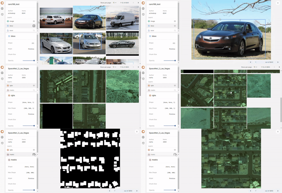
If that is not enough, you probably would find the option to visualize your dataset alongside annotation; without writing a single line of code, is quite tempting to try out this tool. You can do this using the visualizer provided by the app’s friendly interface.

Visualizing two different datasets on Activeloop visualizer
Before We Begin
When I was first introduced to the tool, I wasn’t sure where I can use it, or if it was necessary at all. And I guess this could be the case with all new tools, but at the same time, I was fascinated by the features it offers. I remember asking myself, ok, what is the catch? Honestly, I thought, this is just too good to be true and has so much potential. That what made me quite curious to try it out.
By the end of the project, I realized how powerful it was. In all honesty, I wish that I used it sooner because it did save me a lot of time and unnecessary effort.
The tool is free, open-source, and evolving fast, so there are new features, better implementations, and most importantly, great support from the community and resolving bugs as quickly as possible. But don’t take my word for it. You can join the Slack Community and see for yourself.
Dear reader, please note that what I’m about to share is taken from my experience and does not cover the tool’s full potential. I myself, still learning and discovering new emerging functionalities and implementations for it. Please visit the Hub Repo on GitHub and Documentation for more information and constant updates.
The Rise of the Challenge
During the project we used LandCoverNet which is a labeled, multispectral, and global annual land cover classification training dataset. The data was huge, and we end up downloading a sample of it to train a land cover type classifier. Since we are working with open source and free tools mostly during these types of projects, we ended up training our models mostly on Google Colab and that left us with what seemed to be the obvious and straightforward choice, of storing the data on Google drive. Which proved to be impractical and time-consuming. The data was big so we had to zip it, unzip it before training, do some necessary preprocessing steps before feeding it to the model. This had to be the case every time we wanted to start and train our model.
To add to this challenge we decided to try training a U-Net model and include the extra channel (band) that was included in the dataset, which is the NDVI (Normalised Difference Vegetation Index). We thought that this will provide a better learning opportunity for our model, I’ll go into more details about training the model hopefully in a future blog.
Here we felt the need and obligation to try out Hub and leverage its features.
Activeloop Hub to The Rescue
Read your images into Numpy arrays, store them in Hub and use them anytime, anywhere. It can’t get easier than that.

Photo by Free To Use Sounds on Unsplash
What you need to know is the size of your dataset, the size of the images (dataset with images in different sizes is also supported), and the type. You are all set!
You’ll also need the user name and password for uploading the data. So don’t forget to create an account on the Hub website.
Install Hub
At the time of writing this blog, version 1.3 was the latest version, so this is the one we’ll be installing.
pip3 install hub==1.3
One last thing, you’ll also need to login to Hub using the credentials mentioned earlier using the following line:
!hub login
This is only necessary if you are planning to upload a dataset.
Define The Dataset Object
The following code allows you to prepare the Dataset object which will be populated next, with the data itself.
1import hub
2from hub.schema import Image
3from hub.schema import Tensor
4from hub.schema import Mask
5from hub.schema import Segmentation
6
7# include your user anme and a name for your dataset
8tag = "rasha/landCoverNet_Omdena_Sample"
9# Define youe dataset object
10ds = Dataset(
11 tag,
12 shape=(2512,), # The size of our dataset
13 mode = "w",
14 schema = {
15 # Here we'll define the structure of our data
16 # The input images
17 # (this is a tif image with 4 bands)
18 "inputs": Tensor(
19 (256, 256, 4),
20 dtype="float32"
21 ),
22
23 # The RGB version of our input
24 "rgb_inputs": Image(
25 shape=(256, 256, 3),
26 dtype="uint8"
27 ),
28
29 # The land cover segmentations
30 "masks": Segmentation(
31 shape=(256, 256, 6),
32 dtype="uint8"
33 )
34 },
35)
36
You can think of it as the blueprint that will let Hub know how the structure of your data.
Read the Computer Vision Data into NumPy Arrays
Next, let’s get our actual data and get everything as a NumPy array. Thankfully this doesn’t require a lot of effort.
1inputs_dir = '/content/landcovernet/inputs' # The directory where our input resides
2targets_dir = '/content/landcovernet/targets' # The directory where our target resides
3# First stack all the bands togather
4
5def process_tiffs(inputs_dir, target_dir):
6 data = []
7 sub_dir_list = []
8 images_target = {}
9 stacked_imgs = []
10 list_bands = []
11 for sub_dir in os.listdir(inputs_dir):
12 # Store the images dir and their target
13 sub_dir_list.append(os.path.join(inputs_dir, sub_dir))
14 print(sub_dir_list)
15
16 for image_dir in sub_dir_list:
17 # Get the rgb version
18 rgb = get_rgb(image_dir)
19 custom_img = get_cust_img(image_dir)
20 mask = get_img_mask(targets_dir, image_dir)
21 mask = process_masks(mask) # get the six classes
22 # Dictionary of image and its target in numpy format
23 images_target = {}
24 images_target = {
25 'input' : custom_img,
26 'input_rgb' : rgb,
27 'mask' : mask,
28 }
29
30 stacked_imgs.append(images_target) # list of dict
31
32 return stacked_imgs
33 #return images
34images_target = process_tiffs(inputs_dir, targets_dir)
35
This will put our entire dataset in a Python dictionary as a Numpy array data type. Now, all we need to do is to pass each value to its correspondence that we created in our Hub Dataset.
Uploading the Computer Vision Dataset in Hub format
1# I just extracted the input, rgb, and segmentation to separate arrays for convenience
2inputs = []
3masks = []
4rgb_inputs = []
5for pairs in images_target:
6 inputs.append(pairs["input"])
7 masks.append(pairs["mask"])
8 rgb_inputs.append(pairs["input_rgb"])
9
10# Pass the data to our Dataset instance we created earlier
11for i in range(len(masks)):
12 ds["masks"][i] = masks[i]
13 ds["inputs"][i] = inputs[i]
14 ds["rgb_inputs"][i] = rgb_inputs[i]
15
16# Upload the data to hub
17ds.flush()
18
And that’s pretty much it!
Now you have your data on the cloud, where you and your team will be able to access it from anywhere and as quickly as you could ever wish for.
To use the data I uploaded in this blog, we can load it using the first line of code we wrote. Note: Login is not required.
dataset = Dataset("rasha/landCoverNet_Omdena_Sample")
Now Let’s take a look at our data from the cloud!
1input = ds["rgb_inputs"][1].compute()
2mask = ds["mask"][1].compute()
3pyplot.imshow(input)
4

Sample from LandCoverNet dataset on the Hub server
Conclusion
As you’ve seen the tool is powerful with lots of potentials and being an open-source tool gives it a super engine that keeps it evolving rapidly. There is support for most types of data and annotations out there.
Now, on the other hand, these fast changes could come as confusing in the beginning, but I have to say the great community and support they have, compensate for this healthy and rapid growth. So you don’t just end up getting used to constant updates in some of the features, but you actually start looking forward to them. Also, it is important to note that the tool is much more stable now than when I first started using it.
And don’t worry, I’ll try to cover using the data to train a model in future blogs :)


