The Problem: Accessing Big Public Computer Vision Datasets like Google Objectron
Working on big datasets like Google Objectron should be fun. But it’s usually not. I’ve definitely spent a couple of afternoons on understanding how to access the data instead of training my machine learning models. At times, I also had to worry if my machine fits it in memory or in the storage once I start pre-processing the data. This was a shared sentiment between my team and I, and we created a solution for it. Now, you can access and start working with big datasets like Google Objectron in a matter of seconds.
This comes thanks to Activeloop Hub a new dataset format for AI (allows for storing any type of a dataset as cloud-native NumPy-like arrays). To illustrate how it works, we’ve partnered with Google’s team working on one of Google’s most popular datasets - Google Objectron.
What is Google Objectron Dataset?
Google Objectron is a large dataset containing nearly four million annotated images. The images, annotations and labels along with other metadata has just been transferred and converted to Hub format. After reading this blog post, you will be acquainted with the simplicity of handling terabyte-scale datasets for computer vision.
About Google Objectron Dataset
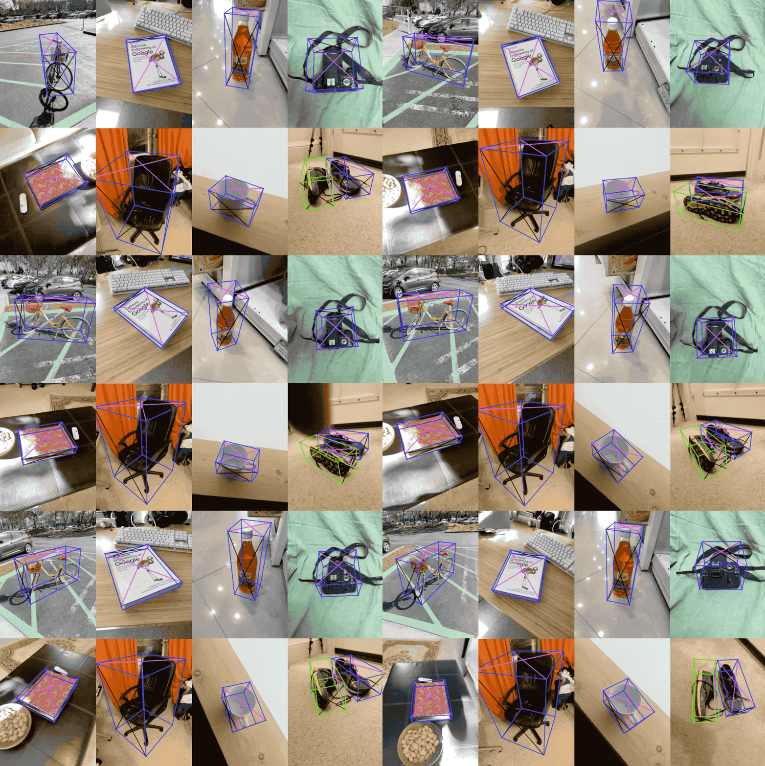
Courtesy of Google Objectron research team*
More specifically, Google Objectron is a dataset representing short video clips of various objects commonly found in modern settings. Developed in 2020 by a team of researchers from Google, the dataset has quickly attracted interest of the open source community. As of March 2021, it is the most popular among all published Google research datasets. It may be speculated that its popularity is driven by the meticulous standards of data collection and annotation as well as the diversity and comprehensibility of the collected images, split in 9 separate categories:
- bike
- book
- bottle
- camera
- cereal_box
- chair
- cup
- laptop
- shoe
These sections include from nearly 500 to over 2000 distinct objects, which translates to approximately 150,000 - 580,000 video frames that can be used in training the machine learning models. The usual way of accessing Objectron data (which involves downloading, parsing and decoding TF Records) may be tedious and time-consuming even for experienced data scientists.
__With Hub, it’s just 28.6 seconds (or a little over 3 seconds per category). __
How to Visualize Google Objectron Dataset?
Before we delve into the data, let’s quickly inspect what’s included in the data with the use of our visualization app. The visualizer is a good starting point for working with any computer vision dataset as it provides you with the schema (information on the data types the dataset is comprised of) and the instructions on how to load the data. Besides, having some intuition with regards to the contents of the data is often required to proceed with the selection of appropriate machine learning solutions to a given problem.
This is how visualizing the bike category of the dataset works. On the left, you may note the schema as well as specific information on a given tensor, including its shape. You may tweak with some of these parameters directly in the app, e.g. you may readily decrease the opacity of a label or an image. Up to 48 images may be represented on a single page. Disclaimer: currently, we’re visualizing just the name and bounding box of the image.

How to access Google Objectron?
You definitely could try downloading the entire Google Objectron Dataset. I’d recommend a smarter approach. Below, I’ll walk you through working with Google Objectron on Hub. You can also play around with the Google Colab notebook we’ve created.
Install the open-source package Hub.
pip install hub
Load the data for bike category.
import hub

bikes_train = hub.dataset("hub://activeloop/objectron_bike_train")
bikes_test = hub.dataset("hub://activeloop/objectron_bike_test")
That’s it, really! You can now access the data as if it were local.
Working with Google Objectron Dataset
The most basic use of Objectron involves browsing through images and their annotations. We need additional tools for some of the visualizations. Please install the following packages:
pip install matplotlib
pip install opencv-python
Then, import these modules.
import matplotlib.pyplot as plt
import cv2
To fetch a sample image with an 4500 index, you may simply run this line of code:
image = bikes_train['image'][4500].numpy()
Then, to plot it, use:
plt.imshow(image, interpolation='nearest')
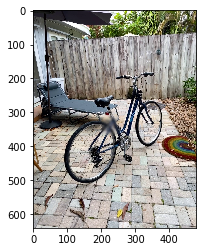
This is the image you should see after running the above code.
Finally, the core value of Objectron are its annotations - 3D bounding boxes. We can represent those with just one function.
def get_bbox(example):
  # Initialize variables
  RADIUS = 10
  COLOR = (255, 255, 255)
  EDGES = [[1, 5], [2, 6], [3, 7], [4, 8],  # lines along x-axis
    [1, 3], [5, 7], [2, 4], [6, 8],  # lines along y-axis
    [1, 2], [3, 4], [5, 6], [7, 8]]   # lines along z-axis

  arranged_points = example['point_2d'].numpy().reshape(9,3)

  # Initialize this variable so that we can add all dots on the image around the box
  image_with_box = example['image'].numpy()

  for i in range(arranged_points.shape[0]):
      x, y, _ = arranged_points[i]
      # Adding the dots on the image around the box
      image_with_box = cv2.circle(image_with_box,(int(x * example['image/width'].numpy()[0]), int(y * example['image/height'].numpy()[0])), RADIUS, COLOR, -10)

  # Now adding the connecting lines between the dots of the box, thus creating the 3D box
  for edge in EDGES:
    start_points = arranged_points[edge[0]]
    start_x = int(example['image/width'].numpy() * start_points[0])
    start_y = int(example['image/height'].numpy() * start_points[1])
    end_points = arranged_points[edge[1]]
    end_x = int(example['image/width'].numpy() * end_points[0])
    end_y = int(example['image/height'].numpy() * end_points[1])
    image_with_box = cv2.line(image_with_box, (start_x, start_y), (end_x, end_y), COLOR, 2)

  plt.imshow(image_with_box)
Fetch the element and pass it to the function to plot the image with the bounding box.
get_bbox(bikes_train[4500])
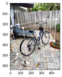
An image of a bike with annotations that you will see after going thorough the guidelines.
You can work with other data categories, like cup, in an identical fashion.
cups = hub.load("hub://activeloop/objectron_cup_train")

cups['image'].shape
which returns: (436513, 640, 480, 3)
Now let’s take a look at the bounding box on the first cup image:
get_bbox(cups_train[0])
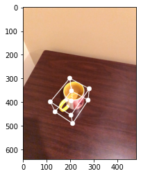
Final Thoughts on Google Objectron Dataset
Well, I hope this was fun. Try to work with the Google Objectron dataset on your own and share your results with us in the Slack community. Feel free to use our Google Objectron notebook to further experiment with Hub. you can also check out our website and documentation to learn more, and join the Slack community to ask our team more questions!
Acknowledgements
We would like to thank Adel Ahmadyan for the support on this project, as well the researchers from Google who developed Objectron, including Liangkai Zhang, Jianing Wei, Artsiom Ablavatski and Matthias Grundmann. Jakub Boros contributed to this blogpost.


